The coursework took me from the mechanics of a robot arm to the uncertainty of a mobile robot. A pose model explains where the mechanism is; mapping and estimation describe the surroundings; planning and behaviour turn that information into a next action. Some of these implementations are mine alone, one went through a paired submission, and the frameworks around them belong to the course.
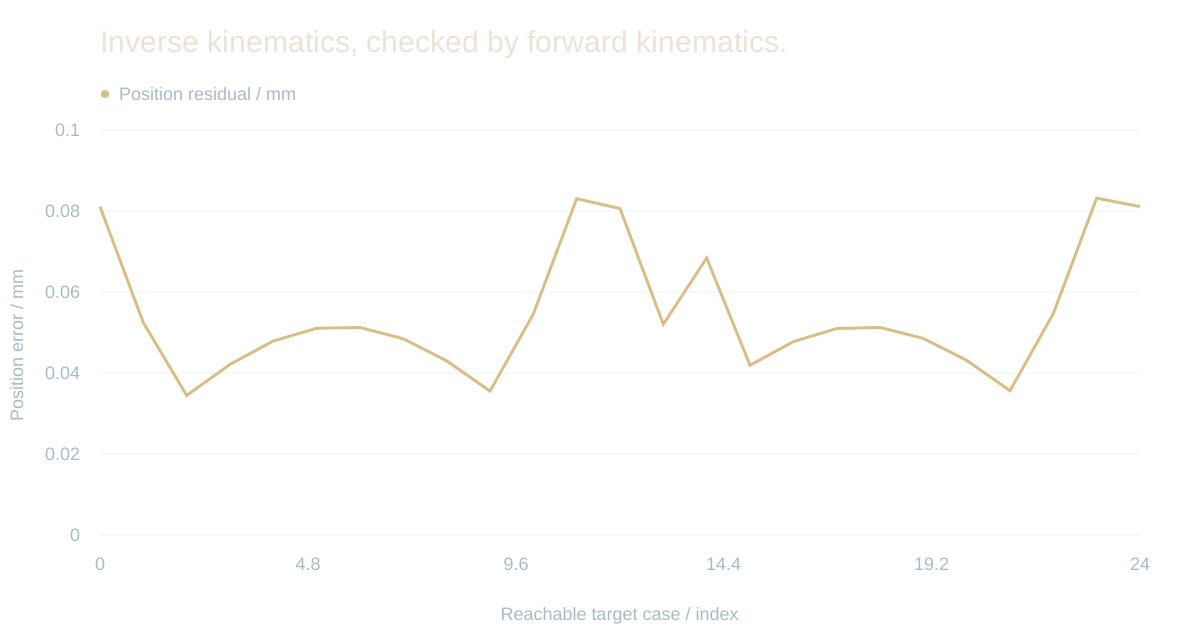
New isolated run of the unchanged submitted IK functions: 25 nearby reachable targets. Forward kinematics checks the solved end pose. No collision, joint-limit or hardware validation is implied.
01 / Forward and inverse kinematics
From joints to a pose. Then solve the reverse.
For the SCARA exercise I used an analytical construction. For the seven-joint KUKA arm I built a transformation chain, a geometric Jacobian and damped least-squares updates that reduce position and orientation error together.
For this page, my unchanged submitted KUKA code was re-run on 25 nearby reachable target poses, with forward kinematics checking each solution. The largest position residual was below 0.084 mm. That is a new local consistency check made for this page, not a historical course benchmark.
INSPECT A SOLVED POSE
01 / 25
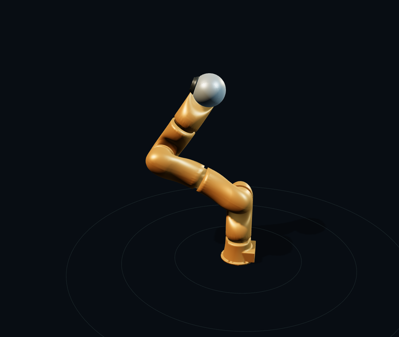
Drag through the solved joint positions. The fine traces retain neighbouring poses, so the arm’s movement stays legible.
Projected joint chain from the original FK code. Geometric illustration; no collision model.
The run and its limits+
My source uses damping 0.01, a 0.5 update step, at most 600 iterations, and 10⁻⁴ tolerances for position and its orientation-error vector. The independent check also evaluates the actual relative rotation angle. The exercise does not validate joint limits, collisions, global convergence or hardware accuracy. The rendered KUKA mesh is the original course model, not custom-designed hardware.
Source: IK_functions.py; course LWR4+ model; new computation-results.json.
A robot-arm simulation shown alongside its terminal. Original monitor recording, 00:06–00:25.
02 / Mapping and estimation
Make free space explicit. Keep uncertainty visible.
The mapping implementation projects laser measurements into a grid, marks ray-traced free space, inserts occupied endpoints and inflates obstacles, so the map is usable by the rest of the navigation stack.
Kalman and extended Kalman filtering belong to the course’s estimation foundation: prediction is corrected by measurement while uncertainty is propagated. The recovered mobile-navigation work uses AMCL, a particle-filter localisation method. I keep those approaches apart rather than presenting one as the other.
Implementation versus course context+
The reviewed mapping.py contains map update and inflation logic. The localisation lecture covers Kalman/EKF concepts. A separate personal Kalman-filter implementation was not established in the recovered submission files, so this page presents it as course knowledge rather than claiming an implemented EKF. The visual map sequence here explains the algorithm; it is not sensor-log playback.
Source: mapping.py; DD2410 mapping materials and localisation lecture.
The obstacle map alongside the simulated environment. Original monitor recording, 00:07–00:24.
03 / Plan a feasible motion
A route must respect how the vehicle turns.
My planner expands a sampling-based tree using bounded steering commands and short forward integrations of a Dubins-style car model. I check obstacle clearance along each segment rather than only at its endpoint.
Goal-biased and Halton samples help explore the space. I attach each new node to its nearest parent without rewiring: the implementation searches for feasible paths and does not claim RRT* optimality.
SAMPLE
Goal bias + low-discrepancy positions
EXTEND
Bounded steering · integrated motion
CHECK
Bounds and inflated obstacles
RETURN
Steering controls and monotonically increasing times
Why the implementation detail matters+
My source includes helpers and comments associated with rewiring, but the executed insertion step explicitly uses the nearest parent only. A feasible returned path and an asymptotically optimal planner are different claims. No completion-rate or optimality benchmark is inferred from the code.
Source: solution.py, sampling, steer_segment and nearest-parent insertion.
04 / Integrate the behaviour
Navigate, recover, continue.
The mobile-robot work combines ROS 2 communication, navigation actions, localisation checks and mission state. Recovery matters when the assumed pose no longer agrees with observations.
This part went through two submissions: an earlier paired one with Nicholas Bosiacki and a later revision I made on my own. Together, the assignments connect arm geometry, mapping and planning to behaviour that responds when the estimated pose no longer fits the observations.
ROS 2
Nodes, topics, services and actions
LOCALISE
AMCL and pose-confidence checks
NAVIGATE
Send a goal and observe its outcome
RECOVER
Reinitialise, gather evidence and resume
Course and contribution record+
Canvas comments distinguish the earlier paired navigation submission with Nicholas Bosiacki from my later individual revision. The arm and planner source files identify my authorship. Course frameworks, provided models and navigation packages retain their original provenance.
Source: BT_students.py, launch/setup files, Canvas submission comments and assignment packages.
The robot and map views changing during a navigation simulation. Original monitor recording, 01:01–01:25.
Guided scroll · scroll or press Escape to take over